氢原子中电子云小记

只接触过大学物理，没学过量子力学，胡乱记录一些基础东西...

在量子力学，通过薛定谔方程可以来理解电子云的分布。氢原子是最简单的原子系统，只有一个质子和一个电子，薛定谔方程可以有解析解。而氦原子有两个电子，就已经超级复杂，只能用近似方法求解了。

概念

粒子的量子态是由波函数 $\psi(\mathbf{r}, t)$ 来描述的。这个波函数包含了这个粒子可能有的一切信息。

spherical_harmonics_y_2_3

薛定谔方程

薛定谔方程是量子力学的基本方程，它描述了量子系统中粒子的波动行为。其一般形式为：

$i\hbar \frac{\partial}{\partial t} \psi(\mathbf{r}, t) = \hat{H} \psi(\mathbf{r}, t)$

其中：

$i$ 是虚数单位，
$\hbar$ 是约化普朗克常数，
$\frac{\partial}{\partial t}$ 是对时间的偏导数，
$\psi(\mathbf{r}, t)$ 是波函数，依赖于位置 $\mathbf{r}$ 和时间 $t$ ，
$\hat{H}$ 是哈密顿算符，它描述了系统的总能量（包括动能和势能）。

对于一个质量为 $m$ 的粒子在势场 $V(\mathbf{r}, t)$ 中运动的情况，哈密顿算符通常可以表示为：

$\hat{H} = -\frac{\hbar^2}{2m} \nabla^2 + V(\mathbf{r}, t)$

其中：

$m$ 是粒子的质量，
$\nabla^2$ 是拉普拉斯算符（描述空间中的二阶导数），
$V(\mathbf{r}, t)$ 是势能函数，依赖于位置和时间。

时间无关薛定谔方程

如果粒子的势能 $V(\mathbf{r})$ 与时间无关，那么，哈密顿算符可以表示

$\hat{H} = -\frac{\hbar^2}{2m} \nabla^2 + V(\mathbf{r}, t)$

可以证明此时薛定谔方程有如下形式的解：

$\psi(\mathbf{r}, t) = \phi(\mathbf{r})\chi(t)$

只考虑 $\phi(\mathbf{r})$ ，薛定谔方程可以简化为时间无关的形式：

$\hat{H}\phi(\mathbf{r}) = E\phi(\mathbf{r})$

其中：

$E$ 是系统的总能量（一个常数），
$\phi(\mathbf{r})$ 是空间依赖的波函数，通常称为定态波函数。

注意，简单起见，后面统一使用符号 $\psi(\mathbf{r})$ 表示此处的 $\phi(\mathbf{r})$

球坐标系

3d_spherical

图片来自wikipedia。

注意此处用的物理中的使用惯例(ISO 80000-2:2019)，和数学中用的惯例的可能不一致。

$r$ 是径向坐标，表示原点到某一点的距离，
$\theta$ 是极角，表示从 $z$ 轴向下的夹角（在 $[0, \pi]$ 的范围内），
$\phi$ 是方位角，表示在 $xy$ 平面内从 $x$ 轴开始的夹角（在 $[0, 2\pi]$ 的范围内）。

在球坐标系 $(r, \theta, \phi)$ 下，拉普拉斯算符 $\nabla^2$ 的形式比直角坐标系中的形式稍微复杂一些。它的具体表达式为：

$\nabla^2 = \frac{1}{r^2} \frac{\partial}{\partial r} \left( r^2 \frac{\partial}{\partial r} \right) + \frac{1}{r^2 \sin \theta} \frac{\partial}{\partial \theta} \left( \sin \theta \frac{\partial}{\partial \theta} \right) + \frac{1}{r^2 \sin^2 \theta} \frac{\partial^2}{\partial \phi^2}$

此时，时间无关的薛定谔方程，变成了：

$-\frac{\hbar^2}{2m} \left( \frac{1}{r^2} \frac{\partial}{\partial r} \left( r^2 \frac{\partial}{\partial r} \right) + \frac{1}{r^2 \sin \theta} \frac{\partial}{\partial \theta} \left( \sin \theta \frac{\partial}{\partial \theta} \right) + \frac{1}{r^2 \sin^2 \theta} \frac{\partial^2}{\partial \phi^2} \right) \psi(r, \theta, \phi) + V(r) \psi(r, \theta, \phi) = E \psi(r, \theta, \phi)$

径向方程与角度方程

使用分离变量法，假设波函数可以分离为径向部分和角度部分：

$\psi(r, \theta, \phi) = R(r) Y(\theta, \phi)$

其中：

$R(r)$ 是径向波函数，
$Y(\theta, \phi)$ 是角度部分波函数（球谐函数）。

代入薛定谔方程后，方程可以分离为两个独立的部分：一个是径向方程，另一个是角度方程。

径向方程：

$\frac{d}{dr} \left( r^2 \frac{dR(r)}{dr} \right) + \left( \frac{2mr^2}{\hbar^2} \left( E - V(r) \right) - l(l+1) \right) R(r) = 0$

这个方程描述了电子在径向方向上的行为，解这个方程可以得到电子在不同能级下的径向波函数。

角度方程：

$\frac{1}{\sin \theta} \frac{\partial}{\partial \theta} \left( \sin \theta \frac{\partial Y(\theta, \phi)}{\partial \theta} \right) + \frac{1}{\sin^2 \theta} \frac{\partial^2 Y(\theta, \phi)}{\partial \phi^2} = -l(l+1) Y(\theta, \phi)$

其解是球谐函数 $Y_l^m(\theta, \phi)$ ，其中 $l$ 是轨道角动量量子数， $m$ 是磁量子数。

球谐函数是定义在球面上的特殊函数，广泛用于物理和数学领域，尤其是在球对称问题中，如量子力学中的原子轨道、经典力学中的引力场和电场，以及计算机图形学中的全局光照。

径向波函数

对于氢原子，前面的径向方程中

$E$ 是电子的能量，与量子数 $n$ 有关。对氢原子来说，能级公式 $E_n=-\frac{13.6\text{eV}}{n^2}$
$V(r) = -\frac{e^2}{4 \pi \epsilon_0 r}$ 是库仑势能，

通过一堆看不懂的数学技巧，最终可以解出来

$R_{n,l}(r) = N_{n,l} \left( \frac{r}{a_0} \right)^l e^{-\frac{r}{n a_0}} L_{n-l-1}^{2l+1} \left( \frac{2r}{n a_0} \right)$

其中：

$L_{n-l-1}^{2l+1} \left( \frac{2r}{n a_0} \right)$ 是拉盖尔多项式，
$n$ 是主量子数，表示电子的能级。
$a_0$ 是波尔半径 $\frac{4 \pi \epsilon_0 \hbar^2}{me^2}$
$N_{n,l}$ 是归一化系数，公式附下面：

$N_{n,l} = \left( \frac{2}{n a_0} \right)^{3/2} \sqrt{\frac{(n - l - 1)!}{2n (n + l)!}}$

这样一来，就可以写python代码了（AI基本可以直接生成）

import numpy as np
from scipy.special import genlaguerre, factorial
from scipy.constants import physical_constants
import matplotlib.pyplot as plt

# Get the Bohr radius a_0
a_0 = physical_constants['Bohr radius'][0]

# Calculate the normalization constant N_{n,l}
def normalization_constant(n, l):
    num = (2 / (n * a_0))**3 * factorial(n - l - 1)
    denom = 2 * n * factorial(n + l)
    return np.sqrt(num / denom)

# Define the radial wavefunction R_{n,l}(r)
def radial_wavefunction(n, l, r):
    rho = 2 * r / (n * a_0)  # Compute the dimensionless variable rho
    laguerre_polynomial = genlaguerre(n - l - 1, 2 * l + 1)  # Generalized Laguerre polynomial
    normalization = normalization_constant(n, l)  # Normalization constant
    radial_part = rho**l * np.exp(-rho / 2) * laguerre_polynomial(rho)  # Main part of the radial wavefunction
    return normalization * radial_part

# Function to plot the radial wavefunction for given n and l
def plot_radial_wavefunction(n, l):
    # Define the range of r values
    r_values = np.linspace(0, 50 * a_0, 1000)  # From 0 to 50 * a_0

    # Compute the radial wavefunction
    R_values = radial_wavefunction(n, l, r_values)

    # Plot the result
    plt.plot(r_values / a_0, R_values, label=f"R_{n},{l}(r)")
    plt.xlabel(r"$r / a_0$")
    plt.ylabel(r"$R_{n,l}(r)$")
    plt.title(f"Radial Wavefunction for n={n}, l={l}")
    plt.grid(True)
    plt.legend()
    plt.show()

# Example usage: Plot for n = 2, l = 0
plot_radial_wavefunction(2, 0)

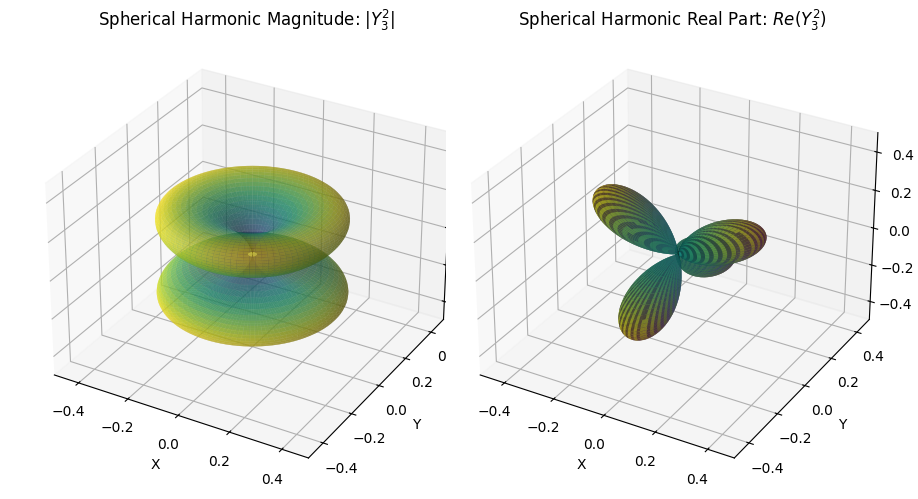
角向波函数（球谐函数）

球谐函数 $Y_{l}^{m}(\theta, \phi)$ 是球坐标系下的两变量函数，定义在角度变量 $\theta$ 和 $\phi$ 上。其一般形式为：

$Y_{l}^{m}(\theta, \phi) = \sqrt{\frac{(2l+1)}{4\pi} \frac{(l-m)!}{(l+m)!}} P_{l}^{m}(\cos\theta) e^{im\phi}$

其中：

$l$ 是非负整数，称为角量子数或多极子阶数。
$m$ 是整数，满足 $-l \leq m \leq l$ ，称为磁量子数。
$\theta$ 是极角，取值范围 $[0, \pi]$ 。
$\phi$ 是方位角，取值范围 $[0, 2\pi]$ 。
$P_{l}^{m}(\cos\theta)$ 是连带勒让德多项式。

这个函数在python中有现成的，所以AI直接给出代码

import numpy as np
import matplotlib.pyplot as plt
from mpl_toolkits.mplot3d import Axes3D
from scipy.special import sph_harm

# Function to visualize both the magnitude and real part of the spherical harmonic
def plot_spherical_harmonic(l, m):
    # Generate the range of angles
    theta = np.linspace(0, np.pi, 100)  # Polar angle θ from 0 to π
    phi = np.linspace(0, 2 * np.pi, 100)  # Azimuthal angle φ from 0 to 2π
    theta, phi = np.meshgrid(theta, phi)  # Create a meshgrid of angles

    # Compute the spherical harmonic Y_l^m(θ, φ)
    Y_lm = sph_harm(m, l, phi, theta)

    # Calculate the magnitude |Y_l^m| (for one plot)
    r_magnitude = np.abs(Y_lm)

    # Calculate the real part Re(Y_l^m) (for the other plot)
    r_real = np.real(Y_lm)

    # Convert spherical coordinates to Cartesian coordinates for magnitude plot
    x_mag = r_magnitude * np.sin(theta) * np.cos(phi)
    y_mag = r_magnitude * np.sin(theta) * np.sin(phi)
    z_mag = r_magnitude * np.cos(theta)

    # Convert spherical coordinates to Cartesian coordinates for real part plot
    x_real = r_real * np.sin(theta) * np.cos(phi)
    y_real = r_real * np.sin(theta) * np.sin(phi)
    z_real = r_real * np.cos(theta)

    # Create a figure with two subplots
    fig = plt.figure(figsize=(16, 6))

    # Subplot 1: Magnitude |Y_l^m|
    ax1 = fig.add_subplot(121, projection='3d')
    ax1.plot_surface(x_mag, y_mag, z_mag, facecolors=plt.cm.viridis(r_magnitude / r_magnitude.max()), 
                     rstride=1, cstride=1, alpha=0.6, edgecolor='none')
    ax1.set_title(f"Spherical Harmonic Magnitude: $|Y_{l}^{m}|$")
    ax1.set_xlim([-0.5, 0.5])
    ax1.set_ylim([-0.5, 0.5])
    ax1.set_zlim([-0.5, 0.5])
    ax1.set_xlabel('X')
    ax1.set_ylabel('Y')
    ax1.set_zlabel('Z')

    # Subplot 2: Real part Re(Y_l^m)
    ax2 = fig.add_subplot(122, projection='3d')
    ax2.plot_surface(x_real, y_real, z_real, facecolors=plt.cm.viridis((r_real - r_real.min()) / (r_real.max() - r_real.min())), 
                     rstride=1, cstride=1, alpha=0.6, edgecolor='none')
    ax2.set_title(f"Spherical Harmonic Real Part: $Re(Y_{l}^{m})$")
    ax2.set_xlim([-0.5, 0.5])
    ax2.set_ylim([-0.5, 0.5])
    ax2.set_zlim([-0.5, 0.5])
    ax2.set_xlabel('X')
    ax2.set_ylabel('Y')
    ax2.set_zlabel('Z')

    # Show the figure
    plt.tight_layout()
    plt.show()

# Example: Plot both magnitude and real part for l = 3, m = 2
plot_spherical_harmonic(3, 2)

spherical_harmonics_y_2_3

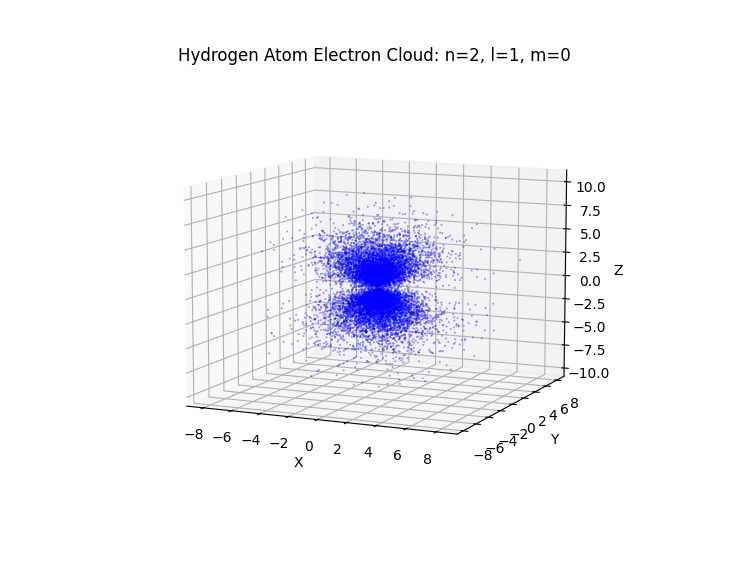
氢原子电子云

电子云图是电子在原子内的概率分布的可视化，它展示了电子在不同位置出现的概率。需要同时考虑径向和角向波函数。概率密度与波函数模平方成正比。

生成随机点（三维坐标下，用球坐标表示）
计算每个点的概率密度（计算波函数模值）
概率筛选（删除概率小的点）
转换为笛卡尔坐标
绘制点云

复数轨道

注意：此处绘制的是复数轨道的模平方，因为球谐函数通常是复数，具有实部和虚部。复数波函数带有相位信息，但其物理含义通常通过波函数模平方来体现。

import numpy as np
import matplotlib.pyplot as plt
from scipy.special import sph_harm, genlaguerre, factorial

# Constants
a0 = 1.0  # Bohr radius (in atomic units)

# Radial wavefunction R_{n,l}(r) for hydrogen atom
def hydrogen_radial_wavefunction(n, l, r):
    # Radial part of the wavefunction for hydrogen atom
    rho = 2 * r / (n * a0)
    # Normalization constant
    norm = np.sqrt((2 / (n * a0))**3 * factorial(n - l - 1) / (2 * n * factorial(n + l)))
    # Radial wavefunction
    radial_part = norm * np.exp(-rho / 2) * rho**l * genlaguerre(n - l - 1, 2 * l + 1)(rho)
    return radial_part

# Probability density function for hydrogen atom
def hydrogen_wavefunction_squared(n, l, m, r, theta, phi):
    # Radial part
    R_nl = hydrogen_radial_wavefunction(n, l, r)
    # Angular part (spherical harmonics)
    Y_lm = sph_harm(m, l, phi, theta)
    # Return the square of the wavefunction (probability density)
    return np.abs(R_nl * Y_lm)**2

# Generate random points in spherical coordinates
def random_points_in_sphere(num_points, n, l, m):
    # Generate random spherical coordinates
    r = np.random.rand(num_points) * 10 * a0  # Random radius within a reasonable range
    theta = np.arccos(2 * np.random.rand(num_points) - 1)  # Uniformly distributed cos(theta)
    phi = np.random.rand(num_points) * 2 * np.pi  # Uniformly distributed phi

    # Compute the probability density at each point
    prob_density = hydrogen_wavefunction_squared(n, l, m, r, theta, phi)

    # Normalize the probabilities
    prob_density /= prob_density.max()

    # Filter points based on probability density (Monte Carlo sampling)
    mask = np.random.rand(num_points) < prob_density

    # Keep only the points that passed the filter
    return r[mask], theta[mask], phi[mask]

# Convert spherical to Cartesian coordinates
def spherical_to_cartesian(r, theta, phi):
    x = r * np.sin(theta) * np.cos(phi)
    y = r * np.sin(theta) * np.sin(phi)
    z = r * np.cos(theta)
    return x, y, z

# Main function to plot the hydrogen atom electron cloud
def plot_hydrogen_cloud(n, l, m, num_points=100000):
    # Generate random points in spherical coordinates
    r, theta, phi = random_points_in_sphere(num_points, n, l, m)

    # Convert spherical coordinates to Cartesian
    x, y, z = spherical_to_cartesian(r, theta, phi)

    # Plot the points
    fig = plt.figure(figsize=(10, 10))
    ax = fig.add_subplot(111, projection='3d')
    ax.scatter(x, y, z, color='blue', s=0.1, alpha=0.6)
    ax.set_xlabel('X')
    ax.set_ylabel('Y')
    ax.set_zlabel('Z')
    ax.set_title(f'Hydrogen Atom Electron Cloud: n={n}, l={l}, m={m}')
    plt.show()

# Example: Plot the electron cloud for the 2p orbital (n=2, l=1, m=0)
plot_hydrogen_cloud(n=2, l=1, m=0)

hydrogen_electron_cloud_2_1_0

实数轨道

实轨道是通过将复数球谐函数的线性组合转换为实数形式来表示的。虽然球谐函数本质上是复数函数，但通过适当的线性组合，可以得到仅包含实数的轨道，这些轨道更符合直观的物理图像。

s-轨道：球对称的，只有 $l=0$ 的情况，没有角动量方向，波函数是实数。

p-轨道：通过将复数球谐函数的线性组合转换为实数形式，我们可以得到三个常用的实轨道 $p_x$ 、 $p_y$ 、 $p_z$ ：

$p_x$ : 对应 $Y_1^1 + Y_1^{-1}$ 的线性组合。（需要归一化？）
$p_y$ : 对应 $Y_1^1 - Y_1^{-1}$ 的线性组合。
$p_z$ : 对应 $Y_1^0$ 。

这些轨道是直观的、方向明确的电子云形状，分别沿着 $x$ 、 $y$ 、 $z$ 轴方向对称。

d-轨道：类似地， $d$ -轨道可以通过 $l=2$ 的复数球谐函数的线性组合得到五个实数轨道，如 $d_{xy}$ 、 $d_{xz}$ 、 $d_{yz}$ 、 $d_{z^2}$ 、 $d_{x^2 - y^2}$ 。

AI给出参考代码如下：

import numpy as np
import matplotlib.pyplot as plt
from scipy.special import sph_harm, factorial

# Constants
a0 = 1.0  # Bohr radius (in atomic units)

# Radial wavefunction R_{n,l}(r) for hydrogen atom
def hydrogen_radial_wavefunction(n, l, r):
    rho = 2 * r / (n * a0)
    norm = np.sqrt((2 / (n * a0))**3 * factorial(n - l - 1) / (2 * n * factorial(n + l)))
    radial_part = norm * np.exp(-rho / 2) * rho**l
    return radial_part

# Probability density function for hydrogen atom
def hydrogen_wavefunction_squared(n, l, m, r, theta, phi):
    R_nl = hydrogen_radial_wavefunction(n, l, r)
    Y_lm = sph_harm(m, l, phi, theta)
    return np.abs(R_nl * Y_lm)**2

# Generate random points in spherical coordinates
def random_points_in_sphere(num_points, n, l, m):
    r = np.random.rand(num_points) * 10 * a0  # Random radius within a reasonable range
    theta = np.arccos(2 * np.random.rand(num_points) - 1)  # Uniformly distributed cos(theta)
    phi = np.random.rand(num_points) * 2 * np.pi  # Uniformly distributed phi
    prob_density = hydrogen_wavefunction_squared(n, l, m, r, theta, phi)

    # Check if max(prob_density) is non-zero before normalizing
    max_density = prob_density.max()
    if max_density > 0:  # Avoid division by zero
        prob_density /= max_density

    # Loosen filtering condition
    mask = np.random.rand(num_points) < prob_density * 5  # Loosen the filtering condition
    print(f"Number of points before filtering: {num_points}, after filtering: {np.sum(mask)}")
    return r[mask], theta[mask], phi[mask]

# Convert spherical to Cartesian coordinates
def spherical_to_cartesian(r, theta, phi):
    x = r * np.sin(theta) * np.cos(phi)
    y = r * np.sin(theta) * np.sin(phi)
    z = r * np.cos(theta)
    return x, y, z

# Real spherical harmonics (p_x, p_y, p_z orbitals)
def real_spherical_harmonics(l, m, theta, phi):
    if l == 1:
        if m == 'p_x':
            # p_x: Re(Y_1^1 + Y_1^-1)
            return (sph_harm(1, 1, phi, theta).real + sph_harm(-1, 1, phi, theta).real)
        elif m == 'p_y':
            # p_y: Im(Y_1^1 - Y_1^-1)
            return (sph_harm(1, 1, phi, theta).imag - sph_harm(-1, 1, phi, theta).imag)
        elif m == 'p_z':
            # p_z: Re(Y_1^0)
            return sph_harm(0, 1, phi, theta).real
    elif l == 2:
        if m == 'd_xy':
            return sph_harm(2, 2, phi, theta).imag
        elif m == 'd_xz':
            return sph_harm(1, 2, phi, theta).real
        elif m == 'd_yz':
            return sph_harm(1, 2, phi, theta).imag
        elif m == 'd_z2':
            return sph_harm(0, 2, phi, theta).real
        elif m == 'd_x2_y2':
            return sph_harm(2, 2, phi, theta).real
    else:
        raise ValueError("Unsupported orbital")

# Main function to plot the hydrogen atom real orbitals
def plot_real_hydrogen_orbital(n, l, m, num_points=100000):
    r, theta, phi = random_points_in_sphere(num_points, n, l, 0)  # m=0, radial sampling
    # Real spherical harmonics
    Y_lm_real = real_spherical_harmonics(l, m, theta, phi)
    prob_density = np.abs(hydrogen_radial_wavefunction(n, l, r) * Y_lm_real)**2

    # Check if max(prob_density) is non-zero before normalizing
    max_density = prob_density.max()
    if max_density > 0:  # Avoid division by zero
        prob_density /= max_density

    # Convert spherical to Cartesian coordinates
    x, y, z = spherical_to_cartesian(r, theta, phi)

    # Plot the points
    fig = plt.figure(figsize=(10, 10))
    ax = fig.add_subplot(111, projection='3d')
    ax.scatter(x, y, z, color='blue', s=0.1, alpha=0.6)
    ax.set_xlabel('X')
    ax.set_ylabel('Y')
    ax.set_zlabel('Z')
    ax.set_title(f'Hydrogen Atom Real Orbital: n={n}, l={l}, m={m}')
    plt.show()

# Example: Plot the real orbital for the p_x orbital (n=2, l=1, m='p_x')
plot_real_hydrogen_orbital(n=2, l=1, m='p_x')

参考

https://liam-ilan.github.io/electron-orbitals/
https://en.wikipedia.org/wiki/Wave_function#Hydrogen_atom
https://ssebastianmag.medium.com/computational-physics-with-python-hydrogen-wavefunctions-electron-density-plots-8fede44b7b12
https://www.researchgate.net/publication/375039550_Quantum_Mechanical_Hydrogen_Atom_Model_Visualised_using_Python
https://physics.stackexchange.com/questions/190726/what-is-the-difference-between-real-orbital-complex-orbital/190730#190730
https://github.com/PyCOMPLETE/PyECLOUD
https://github.com/Niuskir/Electron-Orbitals-Blender-3D
https://github.com/damontallen/Orbitals/blob/master/Hydrogen%20Orbitals%20(Feb%2018,%202014)%20(dynamic%20entry).ipynb
https://in2infinity.com/2d-orbital-geometry-of-the-electron-cloud/

1+1=10

记记笔记，放松一下...